In biological research, particularly in museum-based studies, statistics plays a central role in transforming raw observations into meaningful scientific knowledge. Museum collections and field data provide rich sources of information, ranging from species distributions and ecological patterns to variation in morphological traits across populations. Statistical methods enable researchers to organize, analyze, and interpret these data, uncovering patterns and relationships that would otherwise remain hidden.
This Shiny application is designed as an interactive learning and exploration tool that demonstrates how statistical thinking is applied in real biological and museum research. Through hands-on visualizations and guided examples, users can develop a deeper intuition for key statistical concepts and see how they directly support scientific discovery in the biological sciences.
This resource was developed by the Natural Science Research Laboratory of Museum at Texas Tech. Use the tap panel on the top or below to explore modules designed for High School Statistic Advanced Placement.
📊 Basic Statistics
Quantitative Data
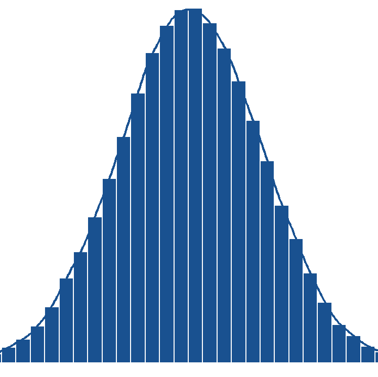 Distribution
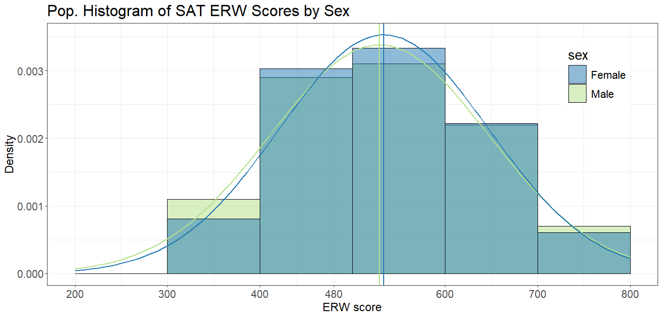
See differences in population distributions
Basic Statistics II
Categorical Data
📈 Linear Regression
See how two variables are related using a line
📊 Inference of Mean(s)
Draw conclusions based on population means
Inference of Proportion(s)
Draw conclusions based on population proportions
🎲 Probability
Likelihood of events
Module 8
Coming soon...
Module 9
Coming soon...
Build your understanding of essential statistical measures—sample size, mean, standard deviation, minimum, maximum, mode, median, and range—using real quantitative data.
Start by exploring the Module 01 PDF for a quick overview or download here. Then strengthen your learning with the interactive app below using provided or your own data!
Explore graphical representations of quantitative data to understand their distribution, shape, and variability.
Build your understanding of essential statistical measures for qualitative (categorical) data, including frequencies and proportions (percentages).
📥 Enter name of category and counts
Options for Barplot
📥 Enter counts for each cell
Options for Barplot
Counts
Percent
Develop your understanding of linear regression by learning how relationships between variables are modeled, interpreted, and used for prediction.
Learn how the slope, intercept, and R² describe and evaluate these relationships.
Choose your source data
Enter two sets of numbers with the SAME length
Learn how to draw conclusions about population means using sample data.
This module includes three sections: one mean, two means, and paired means.
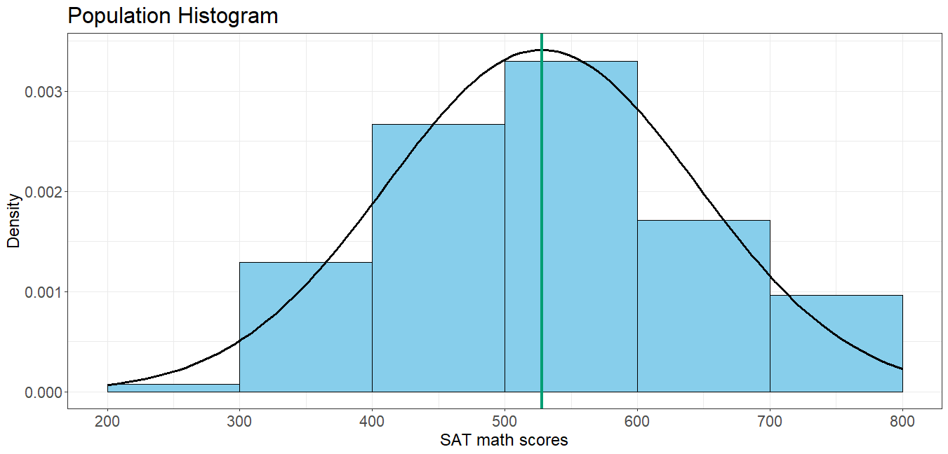
A researcher plans to take a random sample of size n students to do a survey about their experience on the SAT math test. The researcher makes a confidence interval for the SAT math scores of the students in her study and compares it to the mean of 528 for the population of all seniors in the U.S. These data are about College Bound high school graduates in the year of 2019 who participated in the SAT Program. Students are counted only once, no matter how often they tested, and only their latest scores and most recent SAT Questionnaire responses are summarized.
Click the analyze button to create 50 samples to see their confidence intervals and histograms.
Population Information
Population difference in means is -12, Standard deviation for the difference in population means is 163.38
Click the analyze button to draw a new sample from the population
Null hypothesis: (Enter correct \( \mu_D \) value)
Learn how to draw conclusions about population proportions using sample data.
This module includes two sections: one proportion and two proportions.
Null hypothesis: (Enter hypothesized population proportion)
Null hypothesis: (Enter the null value for the difference in proportions)
\( H_0 : p_1 - p_2 = \)
This module introduces the fundamentals of probability through simulation, allowing users to explore random events,
compare empirical and theoretical results, and understand key probability rules.
Select events A and B, then click Analyze button to view questions and answers
Event A
Event B
Simulation Output
Probability Analysis
Event A
Event B
Sample Visualization
Probability Rules
- Initial release